Model diagnostics
Residuals
Recall from module 2, where we looked at residual plots to check our assumptions for a linear model. In a similar way we can use residuals to check how appropriate our GLM is (i.e., to help diagnose the overall goodness-of-fit and to see if our model assumptions are met). Often, Pearson and deviance residuals are used in model diagnostics for generalized linear models.
Response residuals are the conventional residual on the response level. That is, the fitted residuals are transformed by taking the inverse of the link function. Think back to linear models where the link function was set as the identity.
Deviance residuals represent the contributions of individual samples to the deviance, D (see above).
Pearson residuals are calculated by normalizing the raw residuals (i.e., expected - estimate) by the square root of the estimate.
Luckily, we can calculate all three directly in R. Below we do that for the bird abundance model.
## response residuals
resids_response <- residuals(glm_bird, type = "response")
## deviance residuals
resids_deviance <- residuals(glm_bird, type = "deviance")
## pearson residuals
resids_pearson <- residuals(glm_bird, type = "pearson")
Plotting all three types we can asses how appropriate our chosen model is.
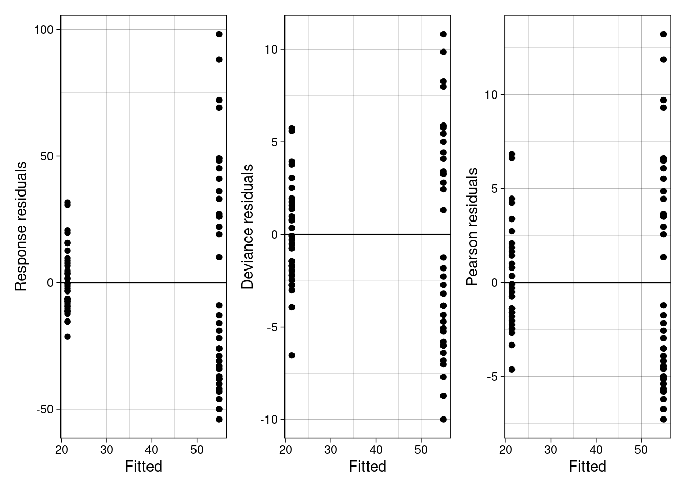
So, what do you see? Look back at the assumptions of a Poisson model. What do you conclude from the plots above?
The quantile residual Q-Q plot
Recall from Module 2 that a Normal quantile-quantile (Q-Q) plot is used to check overall similarity of the observed distribution of the residuals to that expected under the model (i.e., Gaussian). An alternative to a Normal Q-Q plot for a GLM fit is a quantile residual Q-Q plot of observed versus expected quantile residuals. Quantile residuals are, typically, the residuals of choice for GLMs when the deviance and Pearson residuals can be grossly non-normal. It is suggested that quantile residuals are the only useful residuals for binomial or Poisson data when the response takes on only a small number of distinct values. We can use the statmod::qresiduals() function to compute these residuals.
Deviance (using the chi-squared approach)
For our Poisson model
## extract the residual deviance
D <- glm_bird$deviance
D
## [1] 1621.948
## extract the residual degrees of freedom (n-k)
df <- glm_bird$df.residual
df
## [1] 78
Therefore, to test the relevant null hypothesis (that the model is correct) we use
We have strong evidence to reject the null hypothesis; suggesting a lack of fit! BUT are our chi-squared approximation assumptions met? If not, we might take a simulation based approach. This is, however, beyond the scope of this course.
For our binomial model
## extract the residual deviance
D <- glm_mod_gr$deviance
D
## [1] 4.562321
## extract the residual degrees of freedom (n-k)
df <- glm_mod_gr$df.residual
df
## [1] 9
Therefore, to test the relevant null hypothesis (that the model is correct) we use
Here, we have no evidence to against our model being “correct”. BUT are our chi-squared approximation assumptions met? If not, we might take a simulation based approach. This is, however, beyond the scope of this course.