Linear regression
Model formula syntax in R
In R to specify the model you want to fit you typically create a model formula object; this is usually then passed as the first argument to the model fitting function (e.g., lm()).
Some notes on syntax:
Consider the model formula example y ~ x + z + x:z. There is a lot going on here:
- The variable to the left of
~specifies the response, everything to the right specify the explanatory variables +indicated to include the variable to the left of it and to the right of it (it does not mean they should be summed):denotes the interaction of the variables to its left and right
Additional, some other symbols have special meanings in model formula:
*means to include all main effects and interactions, soa*bis the same asa + b + a:b^is used to include main effects and interactions up to a specified level. For example,(a + b + c)^2is equivalent toa + b + c + a:b + a:c + b:c(note(a + b + c)^3would also adda:b:c)-excludes terms that might otherwise be included. For example,-1excludes the intercept otherwise included by default, anda*b - bwould producea + a:b
Mathematical functions can also be directly used in the model formula to transform a variable directly (e.g., y ~ exp(x) + log(z) + x:z). One thing that may seem counter intuitive is in creating polynomial expressions (e.g., x2). Here the expression y ~ x^2 does not relate to squaring the explanatory variable x (this is to do with the syntax ^ you see above. To include x^2 as a term in our model we have to use the I() (the “as-is” operator). For example, y ~ I(x^2)).
| Traditional name | Model formula | R code |
|---|---|---|
| Simple regression | \(Y \sim X_{continuous}\) | lm(Y ~ X) |
| One-way ANOVA | \(Y \sim X_{categorical}\) | lm(Y ~ X) |
| Two-way ANOVA | \(Y \sim X1_{categorical} + X2_{categorical}\) | lm(Y ~ X1 + X2) |
| ANCOVA | \(Y \sim X1_{continuous} + X2_{categorical}\) | lm(Y ~ X1 + X2) |
| Multiple regression | \(Y \sim X1_{continuous} + X2_{continuous}\) | lm(Y ~ X1 + X2) |
| Factorial ANOVA | \(Y \sim X1_{categorical} * X2_{categorical}\) | lm(Y ~ X1 * X2) or lm(Y ~ X1 + X2 + X1:X2) |
Some mathematical notation
Let’s consider a linear regression with a simple explanatory variable:
\[Y_i = \alpha + \beta_1x_i + \epsilon_i\] where
\[\epsilon_i \sim \text{Normal}(0,\sigma^2).\]
Here for observation \(i\)
- \(Y_i\) is the value of the response
- \(x_i\) is the value of the explanatory variable
- \(\epsilon_i\) is the error term: the difference between \(Y_i\) and its expected value
- \(\alpha\) is the intercept term (a parameter to be estimated), and
- \(\beta_1\) is the slope: coefficient of the explanatory variable (a parameter to be estimated)
When we fit a linear model we make some key assumptions:
- Independence
- There is a linear relationship between the response and the explanatory variables
- The residuals have constant variance
- The residuals are normally distributed
In Module 4 you will learn that we have tools that enable us to relax some of these assumptions, after all these assumptions only very rarely hold for real-world data.
In the sections below we use the penguins data from the palmerpenguins package to fit a number of different models using bill Depth (mm) of penguins as the response variable. We first remove the NA values for the response variable:
A Null model
ggplot(data = penguins, aes(x = bill_depth_mm)) +
  geom_histogram() + theme_classic() +
  xlab("Bill depth (mm)")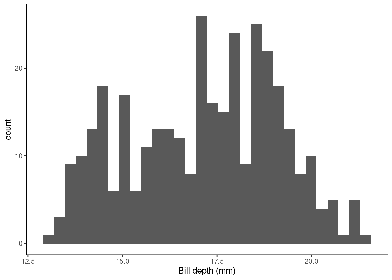
Let’s fit a null (intercept only) model. This in old money would be called a one sample t-test.
slm_null <- lm(bill_depth_mm ~ 1, data = penguins)
summary(slm_null)$coef
##             Estimate Std. Error  t value      Pr(>|t|)
## (Intercept) 17.15117  0.1067846 160.6147 1.976263e-323
Model formula
This model, from above, is simply \[Y_i = \alpha + \epsilon_i.\]
Here for observation \(i\) \(Y_i\) is the value of the response (bill_depth_mm) and \(\alpha\) is a parameter to be estimated (typically called the intercept).
Inference
The (Intercept) term, 17.1511696, tells us the (estimated) average value of the response (bill_depth_mm), see
penguins %>% summarise(average_bill_depth = mean(bill_depth_mm))
## # A tibble: 1 × 1
##   average_bill_depth
##                <dbl>
## 1               17.2
The SEM (Std. Error) = 0.1067846.
The hypothesis being tested is \(H_0:\) ((Intercept) ) \(\text{mean}_{\text{`average_bill_depth`}} = 0\) vs. \(H_1:\) ((Intercept)) \(\text{mean}_{\text{`average_bill_depth`}} \neq 0\)
The t-statistic is given by t value = Estimate / Std. Error = 160.6146593
The p-value is given byPr (>|t|) = 2^{-323}.
So the probability of observing a t-statistic as least as extreme given under the null hypothesis (average bill depth = 0) given our data is 2^{-323}, pretty strong evidence against the null hypothesis I’d say!
Single continuous variable
Does bill_length_mm help explain some of the variation in bill_depth_mm?
p1 <- ggplot(data = penguins, aes(x = bill_length_mm, y = bill_depth_mm)) +
  geom_point() + ylab("Bill depth (mm)") +
  xlab("Bill length (mm)") + theme_classic()
p1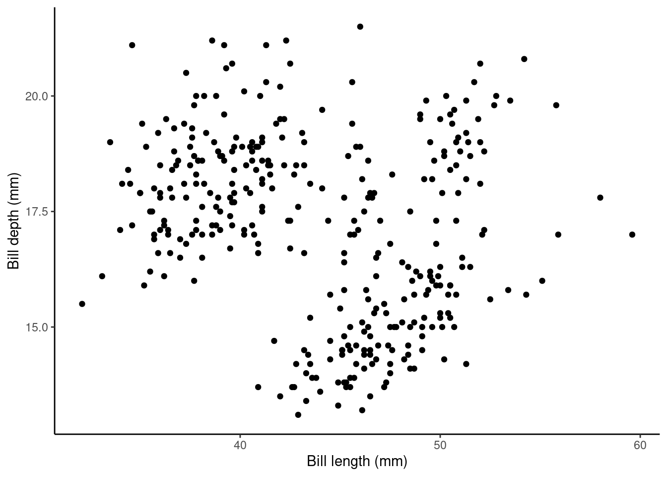
Model formula
This model is simply \[Y_i = \alpha + \beta_1x_i + \epsilon_i\] where for observation \(i\) \(Y_i\) is the value of the response (bill_depth_mm) and \(x_i\) is the value of the explanatory variable (bill_length_mm); As above \(\alpha\) and \(\beta_1\) are parameters to be estimated. We could also write this model as
\[ \begin{aligned} \operatorname{bill\_depth\_mm} &= \alpha + \beta_{1}(\operatorname{bill\_length\_mm}) + \epsilon \end{aligned} \]
Fitted model
As before we extract the estimated parameters (here \(\alpha\) and \(\beta_1\)) using
summary(slm)$coef
##                   Estimate Std. Error   t value     Pr(>|t|)
## (Intercept)    20.88546832 0.84388321 24.749240 4.715137e-78
## bill_length_mm -0.08502128 0.01906694 -4.459093 1.119662e-05
Here, the (Intercept): Estimate (\(\alpha\) above) gives us the estimated average bill depth (mm) given the estimated relationship bill length (mm) and bill length.
The bill_length_mm : Estimate (\(\beta_1\) above) is the slope associated with bill length (mm). So, here for every 1mm increase in bill length we estimated a 0.085mm decrease (or a -0.085mm increase) in bill depth.
## calculate predicted values
penguins$pred_vals <- predict(slm)
## plot
ggplot(data = penguins, aes(x = bill_length_mm, y = bill_depth_mm)) +
  geom_point() + ylab("Bill depth (mm)") +
  xlab("Bill length (mm)") + theme_classic() +
  geom_line(aes(y = pred_vals))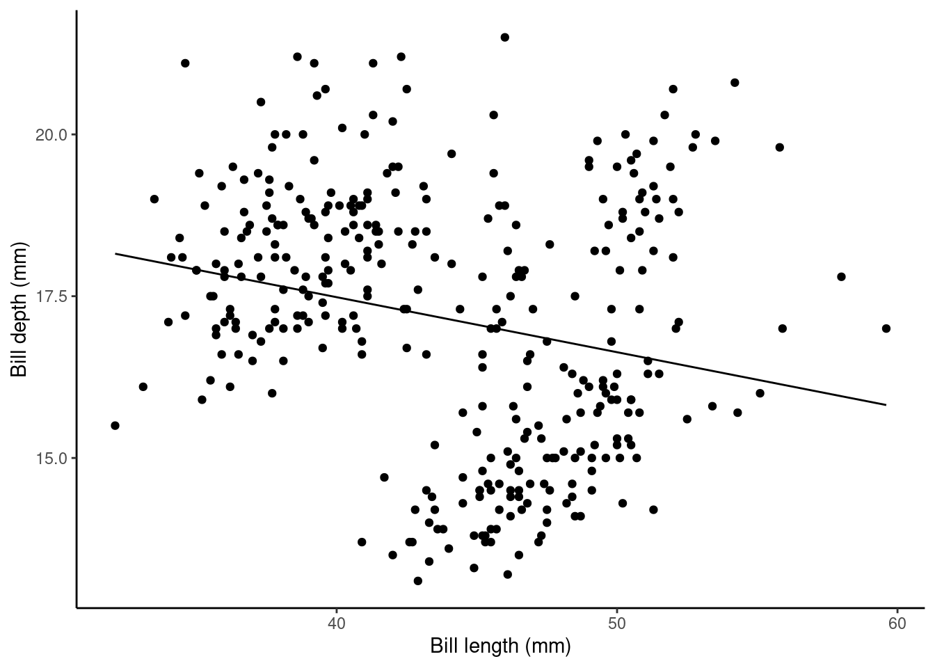
A single factor variable
Does bill_depth_mm vary between species? Think of ANOVA.
p1 <- ggplot(data = penguins, aes(x = species, y = bill_depth_mm)) +
  geom_violin() + ylab("Bill depth (mm)") +
  xlab("Species") + theme_classic() + stat_summary(stat = "mean")
p1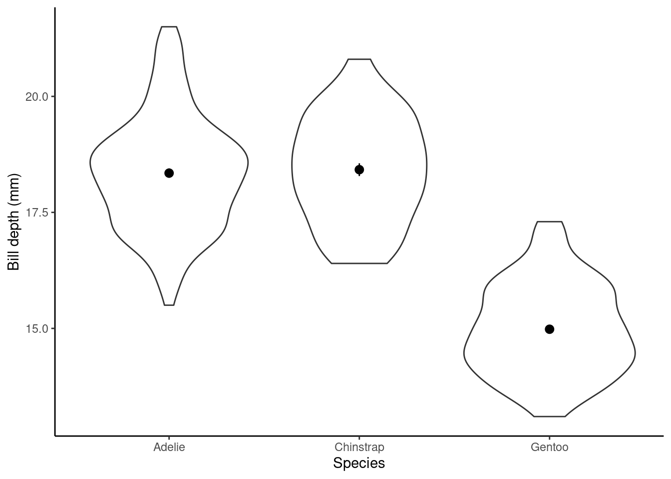
Model formula
This model is simply \[Y_i = \alpha + \beta_1x_i + \epsilon_i\] where for observation \(i\), \(Y_i\) is the value of the response (bill_depth_mm) and \(x_i\) is the value of the explanatory variable (species). However, species is a factor variable. This means we need to use dummy variables:
\[ \begin{aligned} \operatorname{bill\_depth\_mm} &= \alpha + \beta_{1}(\operatorname{species}_{\operatorname{Chinstrap}}) + \beta_{2}(\operatorname{species}_{\operatorname{Gentoo}}) + \epsilon \end{aligned} \]
Fitted model
The estimated parameters (here \(\alpha\), \(\beta_1\), and \(\beta_2\)) are
summary(sflm)$coef
##                     Estimate Std. Error     t value     Pr(>|t|)
## (Intercept)      18.34635762 0.09121134 201.1411914 0.000000e+00
## speciesChinstrap  0.07423062 0.16368785   0.4534889 6.504869e-01
## speciesGentoo    -3.36424379 0.13613555 -24.7124554 7.929020e-78
Here, the (Intercept): Estimate (\(\alpha\) above) gives us the estimated average bill depth (mm) of the baseline species Adelie (R does this alphabetically, to change this see previous chapter) and the remaining coefficients are the estimated difference between the baseline and the other categories (species). The Std. Error column gives the standard error for these estimated parameters (in the case of the group differences there are the SEDs, standard error of the difference).
## calculate predicted values
penguins$pred_vals <- predict(sflm)
## plot
ggplot(data = penguins, aes(x = species, y = bill_depth_mm, fill = species)) +
  geom_violin() + ylab("Bill depth (mm)") +
  xlab("Species") + theme_classic() +
  geom_hline(aes(yintercept = pred_vals, col = species), linewidth = 2) +
    stat_summary(stat = "mean")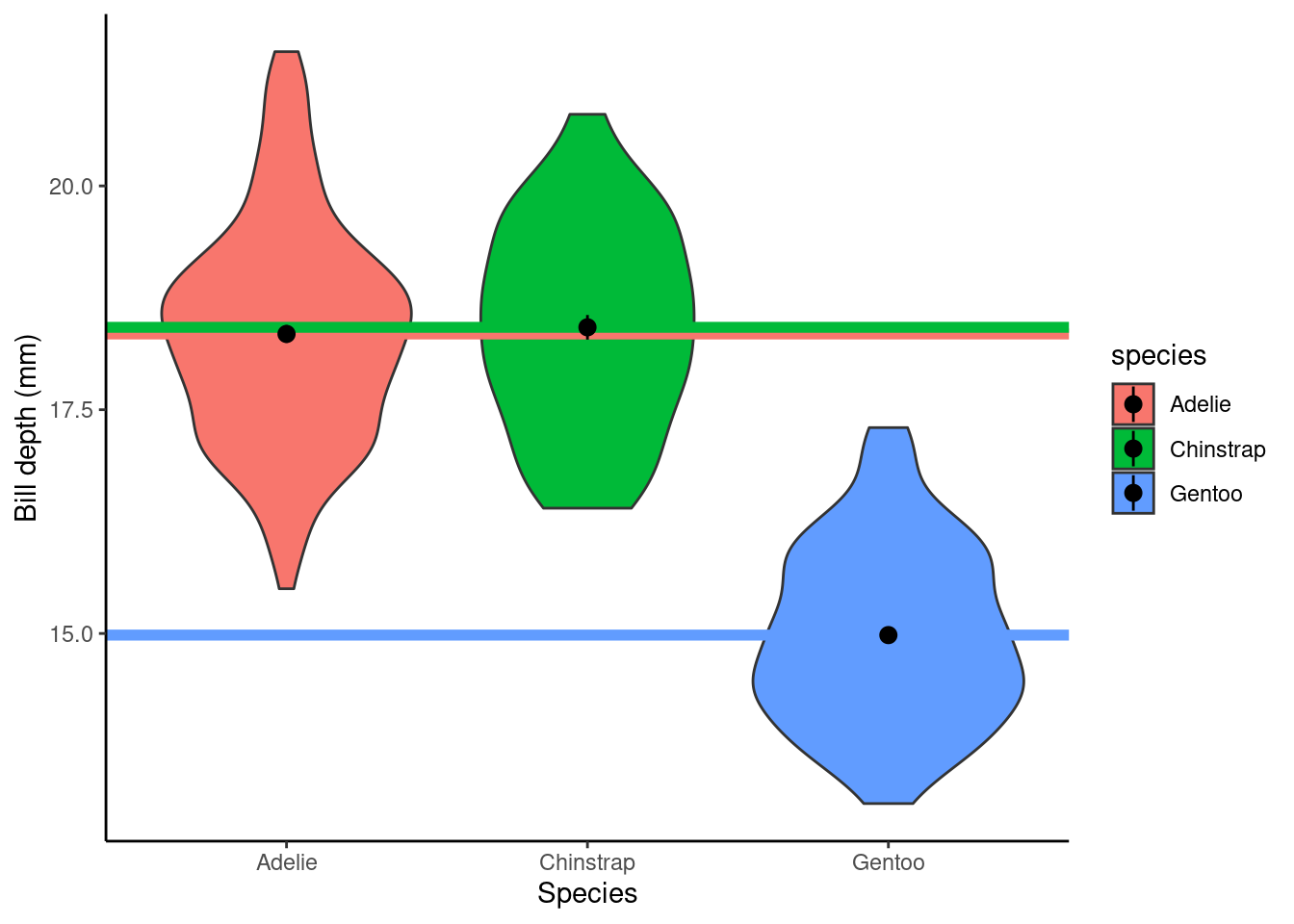
One factor and a continuous variable
p2 <- ggplot(data = penguins,
             aes(y = bill_depth_mm, x = bill_length_mm, color = species)) +
  geom_point() + ylab("Bill depth (mm)") +
  xlab("Bill length (mm)") + theme_classic()
p2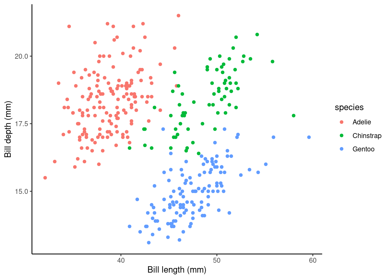
Model formula
Now we have two explanatory variables, so our model formula becomes
\[Y_i = \beta_0 + \beta_1z_i + \beta_2x_i + \epsilon_i\] \[\epsilon_i \sim \text{Normal}(0,\sigma^2)\]
where for observation \(i\)
- \(Y_i\) is the value of the response (
bill_depth_mm) - \(z_i\) is one explanatory variable (
bill_length_mmsay) - \(x_i\) is another explanatory variable (
speciessay) - \(\epsilon_i\) is the error term: the difference between \(Y_i\) and its expected value
- \(\alpha\), \(\beta_1\), and \(\beta_2\) are all parameters to be estimated.
Here, again, the Adelie group are the baseline.
So model formula is
\[ \begin{aligned} \operatorname{bill\_depth\_mm} &= \alpha + \beta_{1}(\operatorname{bill\_length\_mm}) + \beta_{2}(\operatorname{species}_{\operatorname{Chinstrap}}) + \beta_{3}(\operatorname{species}_{\operatorname{Gentoo}})\ + \\ &\quad \epsilon \end{aligned} \]
Fitted model
summary(slm_sp)$coef
##                    Estimate Std. Error   t value     Pr(>|t|)
## (Intercept)      10.5921805 0.68302332  15.50779 2.425034e-41
## bill_length_mm    0.1998943 0.01749365  11.42668 8.661124e-26
## speciesChinstrap -1.9331943 0.22416005  -8.62417 2.545386e-16
## speciesGentoo    -5.1060201 0.19142432 -26.67383 3.650225e-85
Simpson’s paradox… look how the slope associated with bill length (coefficient of bill_length_mm) has switched direction from the model above! Why do you think this is?
Here, the (Intercept): Estimate gives us the estimated average bill depth (mm) of the Adelie penguins given the estimated relationship between bill length and bill depth. Technically, this is the estimated bill depth (mm) for Adelie penguins with zero bill length. That is clearly a nonsense way to interpret this as that would be an impossible situation in practice! I would recommend as thinking of this as the y-shift (i.e., height) of the fitted line.
The bill_length_mm : Estimate (\(\beta_1\) above) is the slope associated with bill length (mm). So, here for every 1mm increase in bill length we estimated a 0.2mm increase in bill depth.
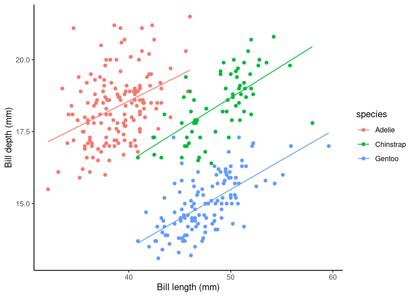
What about the coefficient of the other species levels? Look at the plot below, these values give the shift (up or down) of the parallel lines from the Adelie level. So given the estimated relationship between bill depth and bill length these coefficients are the estimated change from the baseline.
## calculate predicted values
penguins$pred_vals <- predict(slm_sp)
## plot
ggplot(data = penguins, aes(y = bill_depth_mm, x = bill_length_mm, color = species)) +
  geom_point() + ylab("Bill depth (mm)") +
  xlab("Bill length (mm)") + theme_classic()  +
  geom_line(aes(y = pred_vals))
Interactions
Recall the (additive) model formula from above
\[Y_i = \beta_0 + \beta_1z_i + \beta_2x_i + \epsilon_i\]
but what about interactions between variables? For example,
\[Y_i = \beta_0 + \beta_1z_i + \beta_2x_i + \beta_3z_ix_i + \epsilon_i\]
Note: to include interaction effects in our model by using either the * or : syntax in our model formula. For example,
:denotes the interaction of the variables to its left and right, and*means to include all main effects and interactions, soa*bis the same asa + b + a:b.
To specify a model with additive and interaction effects we use
Model formula
The model formula is then
\[ \begin{aligned} \operatorname{bill\_depth\_mm} &= \alpha + \beta_{1}(\operatorname{bill\_length\_mm}) + \beta_{2}(\operatorname{species}_{\operatorname{Chinstrap}}) + \beta_{3}(\operatorname{species}_{\operatorname{Gentoo}})\ + \\ &\quad \beta_{4}(\operatorname{bill\_length\_mm} \times \operatorname{species}_{\operatorname{Chinstrap}}) + \beta_{5}(\operatorname{bill\_length\_mm} \times \operatorname{species}_{\operatorname{Gentoo}}) + \epsilon \end{aligned} \]
Fitted model
summary(slm_int)$coef
##                                    Estimate Std. Error    t value     Pr(>|t|)
## (Intercept)                     11.40912448 1.13812137 10.0245235 7.283046e-21
## bill_length_mm                   0.17883435 0.02927108  6.1095922 2.764082e-09
## speciesChinstrap                -3.83998436 2.05398234 -1.8695313 6.241852e-02
## speciesGentoo                   -6.15811608 1.75450538 -3.5098873 5.094091e-04
## bill_length_mm:speciesChinstrap  0.04337737 0.04557524  0.9517750 3.418952e-01
## bill_length_mm:speciesGentoo     0.02600999 0.04054115  0.6415701 5.215897e-01
This can be written out:
\[ \begin{aligned} \operatorname{\widehat{bill\_depth\_mm}} &= 11.41 + 0.18(\operatorname{bill\_length\_mm}) - 3.84(\operatorname{species}_{\operatorname{Chinstrap}}) - 6.16(\operatorname{species}_{\operatorname{Gentoo}})\ + \\ &\quad 0.04(\operatorname{bill\_length\_mm} \times \operatorname{species}_{\operatorname{Chinstrap}}) + 0.03(\operatorname{bill\_length\_mm} \times \operatorname{species}_{\operatorname{Gentoo}}) \end{aligned} \]
The interaction terms (i.e., bill_length_mm:speciesChinstrap and bill_length_mm:speciesGentoo) specify the species specific slopes given the other variables in the model. We can use our dummy variable trick again to interpret the coefficients correctly. In this instance we have one factor explanatory variable, Species, and one continuous explanatory variable, bill length (mm). As before, Adelie is our baseline reference.
Let’s assume we’re talking about the Adelie penguins, then our equation becomes (using the dummy variable technique)
\[\widehat{\text{bill_depth_mm}} = 11.409 + (0.179 \times \text{bill_length_mm}).\]
So, the (Intercept): Estimate term (\(\hat{\alpha}\)), again, specifies the height of the Adelie fitted line and the main effect of bill_length_mm: Estimate (\(\hat{\beta_1}\)) estimates the relationship (slope) between bill length (mm) and bill depth (mm) for the Adelie penguin. So, here for every 1mm increase in bill length (mm) for the Adelie penguins we estimate, on average, a 0.179mm increase in bill depth (mm).
Now, what about Gentoo penguins? Our equation then becomes
\[\widehat{\text{bill_depth_mm}} = 11.409 + (0.179 \times \text{bill_length_mm}) + (-6.158) + (0.026 \times \text{bill_length_mm}).\]
which simplifies to
\[\widehat{\text{bill_depth_mm}} = 5.251 + (0.205 \times \text{bill_length_mm}).\]
The estimated Gentoo-specific intercept term (y-axis line height) is therefore \(\hat{\alpha} + \hat{\beta_3} = 11.409 + (-6.158) = 5.251.\) The Gentoo-specific bill length (mm) slope is then \(\hat{\beta_1} + \hat{\beta_5} = 0.179 + 0.026 = 0.205.\) So, for every 1mm increase in bill length (mm) for the Gentoo penguins we estimate, on average, a 0.205mm increase in bill depth (mm), a slightly steeper slope than for the estimated Adelie relationship (i.e., we estimate that as Gentoo bills get longer their depth increases at a, slightly, greater rate than those of Adelie penguins).
In summary, the main effect of species (i.e., speciesChinstrap: Estimate and speciesGentoo:Estimate ) again give the shift (up or down) of the lines from the Adelie level. However, these lines are no longer parallel (i.e., each species of penguin has a different estimated relationship between bill length and bill depth)!
But, now we’ve specified this all singing and dancing interaction model we might ask are the non-parallel lines non-parallel enough to reject the parallel line model? Look at the plot below; what do you think?

Other possible relationships
Let’s assume that we have the same data types as above, specifically, a continuous response (\(y\)) and one factor (\(f\), with two levels \(A\) and \(B\)) and one continuous (\(x\)) explanatory variable. Assuming that \(A\) is the baseline for \(f\) the possible models are depicted below.
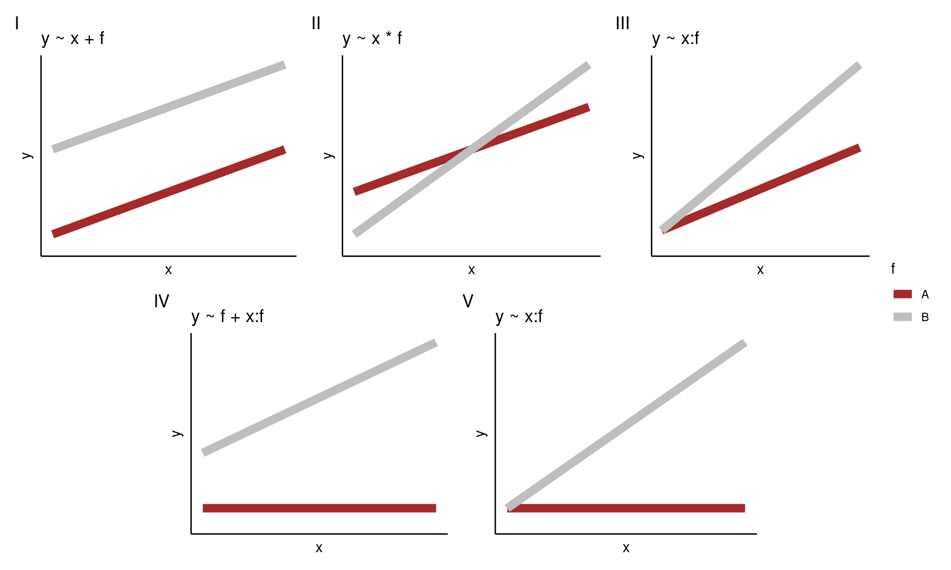
Note that models III and V are forced to have the same intercept for both levels of \(f\). In addition, when you have no main effect of \(x\), models IV and V, then the model is forced to have no effect of \(x\) for the baseline level of \(f\) (in this case \(A\)).