Generalised linear mixed-effects models (GLMMMs)

Recall module 3 when we covered fitting linear models with random effects (lmer). The fixed effects and random effects were specified via the model formula. Now we’ve covered GLMs we can include random effects here too and fit GLMMs!

Recall

• Fixed effects: terms (parameters) in a statistical model which are fixed, or non-random, quantities (e.g., treatment group’s mean response). For the same treatment, we expect this quantity to be the same from experiment to experiment.
• Random effects: terms (parameters) in a statistical model which are considered as random quantities or variables (e.g., block id). Specifically, terms whose levels are a representative sample from a population, and where the variance of the population is of interest should be allocated as random. Setting a block as a random effect allows us to infer variation between blocks as well as the variation between experimental units within blocks.

Fitting a GLMM

The authors of this paper transplanted gut microbiota from human donors with Autism Spectrum Disorder (ASD) or typically developing (TD) controls into germ-free mice. Faecal samples were collected from three TD and five ASD donors and were used to colonise GF male and female mice from strain C57BL/6LJ. Individuals colonized by the same donor were allowed to breed. Adult offspring mice were behavior tested; tests included marble burying (MB), open-field testing (OFT), and ultrasonic vocalization (USV).

glimpse(mice)
## Rows: 206
## Columns: 3
## $ Donor     <chr> "C1", "C1", "C1", "C1", "C1", "C1", "C1", "C1", "C1", "A24-n…
## $ Treatment <chr> "NT Female", "NT Female", "NT Female", "NT Female", "NT Male…
## $ MB_buried <dbl> 3, 8, 1, 3, 2, 6, 4, 2, 9, 7, 5, 5, 11, 13, 6, 14, 9, 5, 6, …

We should separate out the treatment values:

mice <- mice %>%
  separate(., col = Treatment, into = c("Diagnosis", "Sex"))
mice
## # A tibble: 206 × 4
##    Donor   Diagnosis Sex    MB_buried
##    <chr>   <chr>     <chr>      <dbl>
##  1 C1      NT        Female         3
##  2 C1      NT        Female         8
##  3 C1      NT        Female         1
##  4 C1      NT        Female         3
##  5 C1      NT        Male           2
##  6 C1      NT        Male           6
##  7 C1      NT        Male           4
##  8 C1      NT        Male           2
##  9 C1      NT        Female         9
## 10 A24-new ASD       Male           7
## # ℹ 196 more rows

Recall, using lmer to fit a LMM

lmer <- lmerTest::lmer(MB_buried ~ Sex * Diagnosis + (1|Donor), data = mice)
car::Anova(lmer, type = 2)
## Analysis of Deviance Table (Type II Wald chisquare tests)
## 
## Response: MB_buried
##                Chisq Df Pr(>Chisq)   
## Sex           3.6329  1   0.056648 . 
## Diagnosis     8.6944  1   0.003192 **
## Sex:Diagnosis 2.9745  1   0.084588 . 
## ---
## Signif. codes:  0 '***' 0.001 '**' 0.01 '*' 0.05 '.' 0.1 ' ' 1

But is the constant error variance appropriate? Below we plot the model residuals.

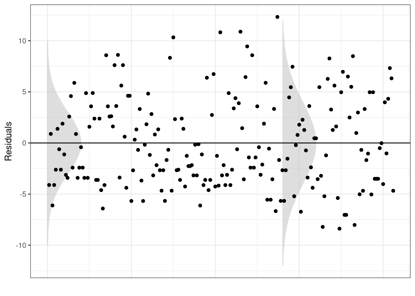
TASK Looking at the output above, do you think the assumptions of the linear model are met?

Using glmer

glmer <- lme4::glmer(MB_buried ~ Sex * Diagnosis + (1|Donor), data = mice, family = poisson(link = "log"))
car::Anova(glmer, type = 2)
## Analysis of Deviance Table (Type II Wald chisquare tests)
## 
## Response: MB_buried
##                 Chisq Df Pr(>Chisq)    
## Sex            9.9452  1  0.0016127 ** 
## Diagnosis     10.5836  1  0.0011410 ** 
## Sex:Diagnosis 12.5904  1  0.0003877 ***
## ---
## Signif. codes:  0 '***' 0.001 '**' 0.01 '*' 0.05 '.' 0.1 ' ' 1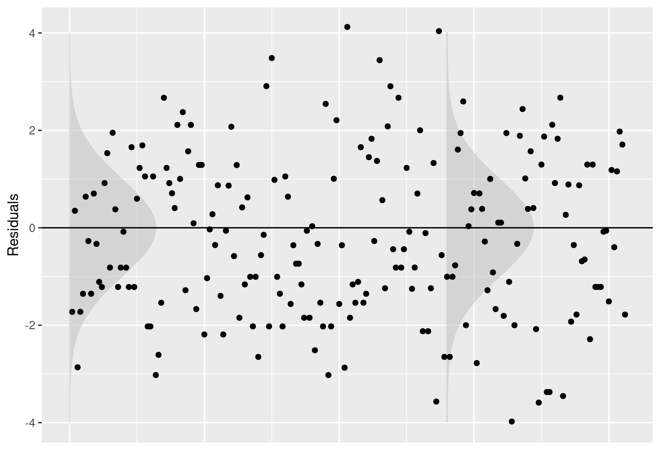

TASK Looking at the output above, do you think the assumptions of the Poisson model are met?