Bootstrap resampling
A sampling distribution shows us what would happen if we took very many samples under the same conditions. The bootstrap is a procedure for finding the (approximate) sampling distribution from just one sample.
The original sample represents the distribution of the population from which it was drawn. Resamples, taken with replacement from the original sample are representative of what we would get from drawing many samples from the population (the distribution of the statistics calculated from each resample is known as the bootstrap distribution of the statistic). The bootstrap distribution of a statistic represents that statistic’s sampling distribution.
TASK Study this cheatsheet and link the relevant sections to each step given above.
Example: constructing bootstrap confidence intervals
Old faithful is a gyser located in Yellowstone National Park, Wyoming. Below is a histogram of the duration of 299 consecutive eruptions. Clearly the distribution is bimodal (has two modes)!
ggplot(data = geyser, aes(x = duration)) +
  geom_histogram() +
  xlab("Duration of eruptions (m)") +
  theme_linedraw()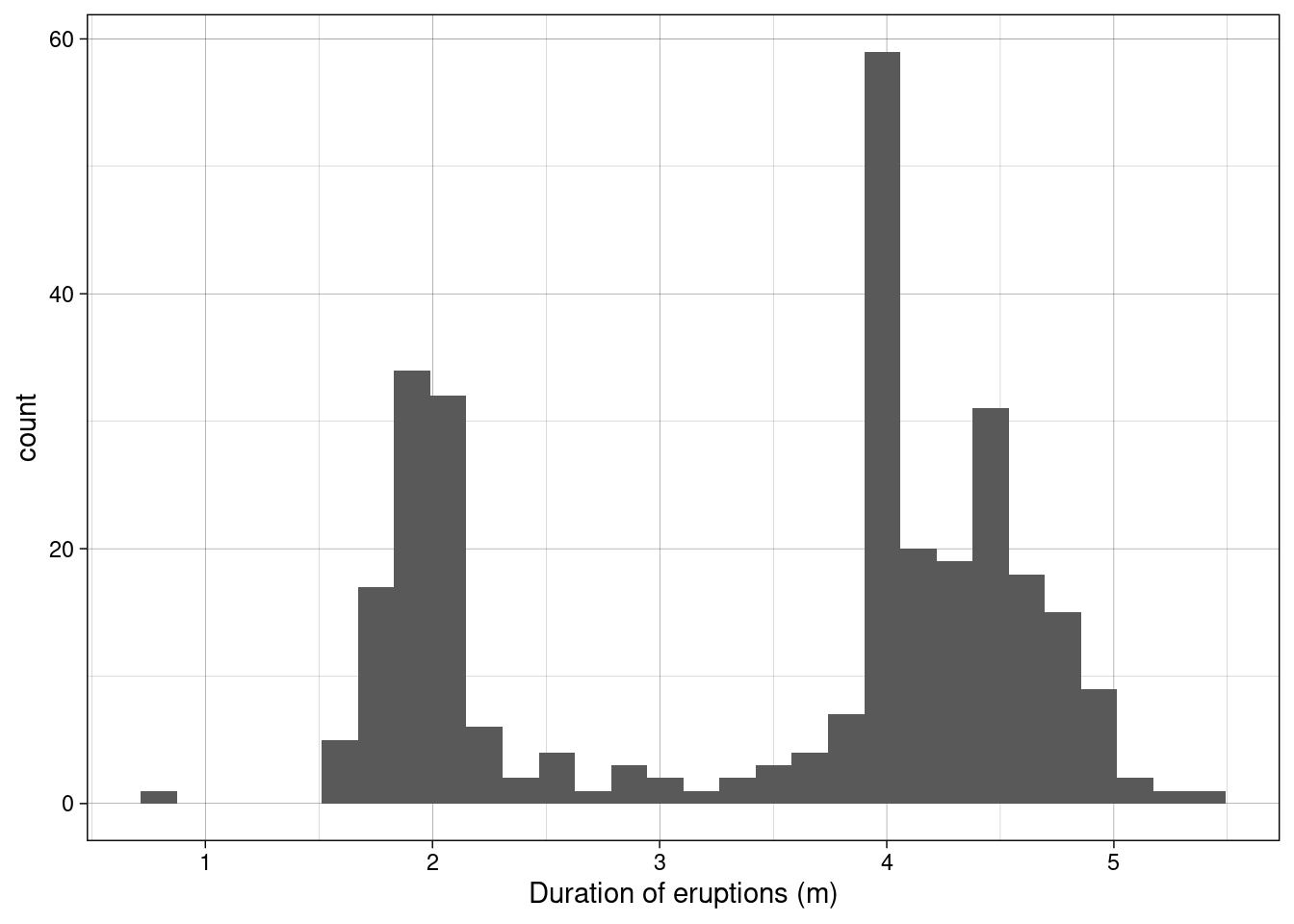
Step 1: Calculating the observed mean eruption duration time:
Step 2: Construct bootstrap distribution
## Number of times I want to bootstrap
nreps <- 1000
## initialize empty array to hold results
bootstrap_means <- numeric(nreps)
set.seed(1234) ## *****Remove this line for actual analyses*****
## This means that each run with produce the same results and
## agree with the printout that I show.
for (i in 1:nreps) {
  ## bootstrap. note with replacement
  bootstrap_sample <- sample(geyser$duration, replace = TRUE)
  ##  bootstrapped mean resample
  bootstrap_means[i] <- mean(bootstrap_sample)
}
Step 3: Collate the sampling distribution
## results
results <- data.frame(bootstrap_means = bootstrap_means)
ggplot(data = results, aes(x = bootstrap_means)) +
  geom_histogram() +
  geom_vline(xintercept = as.numeric(mean)) +
  ggtitle("Sampling distribution of the mean") +
  xlab("Bootstrap means")  + ylab("") + theme_classic()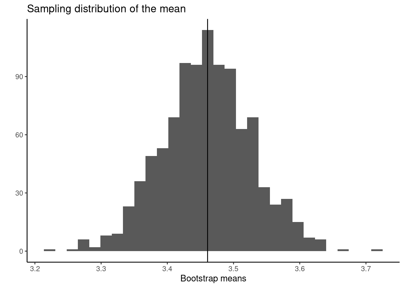
Step 4: Calculate quantities of interest from the sampling distribution
- The bootstrap estimate of bias is the difference between the mean of the bootstrap distribution and the value of the statistic in the original sample:
- The bootstrap standard error of a statistic is the standard deviation of its bootstrap distribution:
sd(results$bootstrap_means)
## [1] 0.06740607
## compare to SEM of original data
 MASS::geyser %>%
  summarise(sem = sd(duration)/sqrt(length(duration)))
##          sem
## 1 0.06638498- A Bootstrap \(t\) confidence interval. If, for a sample of size \(n\), the bootstrap distribution is approximately Normal and the estimate of bias is small then an approximate \(C\) confidence for the parameter corresponding to the statistic is:
\[\text{statistic} \pm t^* \text{SE}_\text{bootstrap}\] where \(t*\) is the critical value of the \(t_{n-1}\) distribution with area \(C\) between \(-t^*\) and \(t^*\).
For \(C = 0.95\):
So our 95% confidence interval is 3.3 to 3.6.
- A bootstrap \(percentile\) confidence interval. Use the bootstrap distribution itself to determine the limits of the confidence interval by taking the limits of the sorted, central \(C\) bulk of the distribution. For \(C = 0.95\):

Resampling procedures, the differences
Resampling methods are any of a variety of methods for doing one of the following
- Estimating the precision of sample statistics (e.g., bootstrapping)
- Performing significance tests (e.g., permutation/exact/randomisation tests)
- Validating models (e.g., bootstrapping, cross validation)
Permutation vs bootstrap test
The permutation test exploits symmetry under the null hypothesis.
A full permutation test p-value is exact, conditional on data values in the combined sample.
A bootstrap estimates the probability mechanism that generated the samples under the null hypothesis.
A bootstrap does not rely on any special symmetry or assumption or exchangeability.